MTH 221: Linear Algebra at The American University of Sharjah
1.
List of concepts and definitions
Back to the main
page (home)
2.
For Examples that Illustrate some of the
concepts Click here (Linear Algebra Tool Kit)
3. Important RESULTS (THEOREMS)(See the
Table Below):
Back to the MAIN PAGE of Ayman Badawi
Eiginvalues and eigenspaces
result
Have you ever heard the words eigenvalue and eigenvector? They are
derived from the German word "eigen" which means "proper" or
"characteristic." An eigenvalue of a square matrix is a scalar that is
usually represented by the Greek letter
 (pronounced lambda). As you might suspect, an eigenvector is a vector.
Moreover, we require that an eigenvector be a non-zero vector, in other
words, an eigenvector can not be the zero vector. We will denote an
eigenvector by the small letter x. All eigenvalues and
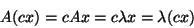
eigenvectors satisfy the equation
(pronounced lambda). As you might suspect, an eigenvector is a vector.
Moreover, we require that an eigenvector be a non-zero vector, in other
words, an eigenvector can not be the zero vector. We will denote an
eigenvector by the small letter x. All eigenvalues and
eigenvectors satisfy the equation
 for a given square matrix, A.
Remark 27 Remember that, in general, the word scalar is not
restricted to real numbers. We are only using real numbers as
scalars in this book, but eigenvalues are often complex numbers.
Definition 9.1 Consider the square matrix A . We say
that
is an eigenvalue of A if
there exists a non-zero vector x such that
.
In this case, x is called an
eigenvector (corresponding to
),
and the pair (,x)
is called an eigenpair for A.
Let's look at an example of an eigenvalue and eigenvector. If you
were asked if
 is an eigenvector corresponding to the eigenvalue
 for
for
 ,
you could find out by substituting x,
and A into the equation ,
you could find out by substituting x,
and A into the equation

Therefore,
and x are an eigenvalue and an eigenvector, respectively, for
A.
Now that you have seen an eigenvalue and an eigenvector, let's talk a
little more about them. Why did we require that an eigenvector not be
zero? If the eigenvector was zero, the equation
would yield 0 = 0. Since this equation is always true, it is not an
interesting case. Therefore, we define an eigenvector to be a non-zero
vector that satisfies
However, as we showed in the previous example, an eigenvalue can be zero
without causing a problem. We usually say that x is an
eigenvector corresponding to the eigenvalue
if they satisfy
Since each eigenvector is associated with an eigenvalue, we often refer
to an x and
that correspond to one another as an eigenpair.
Did you notice that we called x "an" eigenvector rather than
"the" eigenvector corresponding to
?
This is because any non-zero, scalar multiple of an eigenvector is also
an eigenvector. If you let c represent a scalar, then we can
prove this fact through the following steps.
Since any non-zero, scalar multiple of an eigenvector is also an
eigenvector,
 and
and
 are also eigenvectors corresponding to
when
are also eigenvectors corresponding to
when

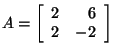
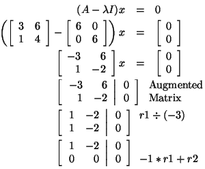
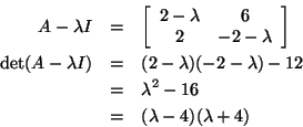
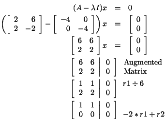
Let's find both of the eigenvalues of the matrix
Therefore,
 or
or
 We now know our eigenvalues. Remember that all eigenvalues are paired
with an eigenvector. Therefore, we can substitute our eigenvalues, one
at a time, into the formula
We now know our eigenvalues. Remember that all eigenvalues are paired
with an eigenvector. Therefore, we can substitute our eigenvalues, one
at a time, into the formula
 and solve to find a corresponding eigenvector.
Let's find an eigenvector corresponding to

Notice that this system is underdetermined. Therefore, there are an
infinite number of solutions. So, any vector that solves the equation
x1 - 2x2 = 0 is an eigenvector
corresponding to
when
To have a consistent method for finding an eigenvector, let's choose the
solution in which x2 = 1. We can use back-substitution
to find that x1 - 2(1) = 0 which implies that x1
= 2. This tells us that
 is an eigenvector corresponding to
when
This is the same solution that we found when we used the power method to
find the dominant eigenpair.
is an eigenvector corresponding to
when
This is the same solution that we found when we used the power method to
find the dominant eigenpair.
Let's find an eigenvector corresponding to
Notice that this system is underdetermined. This will always be true
when we are finding an eigenvector using this method. So, any vector
that solves the equation x1 + 3x2 =
0 is an eigenvector corresponding to the eigenvalue
 when
Again, let's choose the eigenvector in which the last element of x
is 1. Therefore, x2 = 1 and x1 +
3(1) = 0, so x1 = -3. This tells us that
when
Again, let's choose the eigenvector in which the last element of x
is 1. Therefore, x2 = 1 and x1 +
3(1) = 0, so x1 = -3. This tells us that
 is an eigenvector corresponding to
 when
Using the characteristic equation and Gaussian elimination, we are able
to find all the eigenvalues to the matrix and corresponding
eigenvectors.
when
Using the characteristic equation and Gaussian elimination, we are able
to find all the eigenvalues to the matrix and corresponding
eigenvectors.
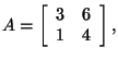
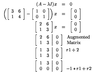
Let's find the eigenpairs for the matrix
 . .
Therefore,
 or
or
 . .
Let's find an eigenvector corresponding to

Since the system is underdetermined, we have an infinite number of
solutions. Let's choose the solution in which x2 = 1.
We can use back-substitution to find that x1 - 3(1 ) =
0 which implies that x1 = 3. This tells us that
 is an eigenvector corresponding to
when
is an eigenvector corresponding to
when
Let's find an eigenvector corresponding to
Again, let's choose the eigenvector in which the last element of x
is 1. Therefore, x2 = 1 and x1 +
1(1) = 0, so x1 = -1. This tells us that
 is an eigenvector corresponding to
when
Using the characteristic equation and Gaussian elimination, we are able
to find both of the eigenvalues to the matrix and corresponding
eigenvectors.
is an eigenvector corresponding to
when
Using the characteristic equation and Gaussian elimination, we are able
to find both of the eigenvalues to the matrix and corresponding
eigenvectors.
We can find eigenpairs for larger systems using this method, but the
characteristic equation gets impossible to solve directly when the
system gets too large. We could use approximations that get close to
solving the characteristic equation, but there are better ways to find
eigenpairs that you will study in the future. However, these two methods
give you an idea of how to find eigenpairs.
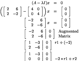
Another matrix for which the power method will not work is the matrix
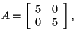 because the eigenvalues are both the real number 5. The method that we
showed you earlier will yield the eigenvector
because the eigenvalues are both the real number 5. The method that we
showed you earlier will yield the eigenvector
 to correspond to the eigenvalue
 .
Other methods will reveal, and you can check, that .
Other methods will reveal, and you can check, that
 is also an eigenvector of A corresponding to
.
Notice that these two eigenvectors are not multiples of one another. If
the same eigenvalue is repeated p times for a particular matrix,
then there can be as many as p different eigenvectors that are
not multiples of each other that correspond to that eigenvalue.
is also an eigenvector of A corresponding to
.
Notice that these two eigenvectors are not multiples of one another. If
the same eigenvalue is repeated p times for a particular matrix,
then there can be as many as p different eigenvectors that are
not multiples of each other that correspond to that eigenvalue.
We said that eigenvalues are often complex numbers. However, if the
matrix A is symmetric, then the eigenvalues will always be real
numbers. As you can see from the problems that we worked, eigenvalues
can also be real when the matrix is not symmetric, but keep in mind that
they are not guaranteed to be real.
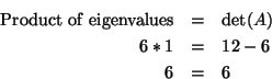
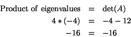
Did you know that the determinant of a matrix is related to the
eigenvalues of the matrix? The product of the eigenvalues of a square
matrix is equal to the determinant of that matrix. Let's look at the two
matrices that we have been working with. For
For

You can use this as a check to see that you have the correct eigenvalues
and determinant for the matrix A.
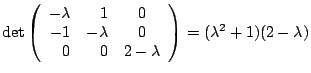
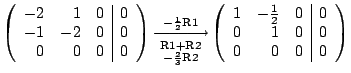
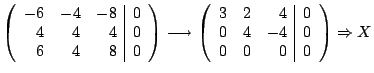
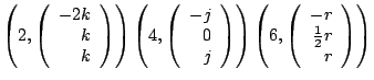
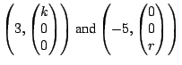
Example Show that
has only one real eigenvalue. Find the eigenspace corresponding to
that eigenvalue.
Solution The characteristic polynomial is
Since  is never zero for real
  is the only real eigenvalue. The eigenvector is found by solving
  with
with
 : :
The general solution is
and the eigenpair is
The eigenspace
Solution The characteristic polynomial
 is
is
To solve  ,
we first guess at one root of .
First we try integer factors of 48: ,
we first guess at one root of .
First we try integer factors of 48:
 , ,
 , ,
 , ,
 , ,
 , ,
 , ,
 , ,
 , ,
 , ,
 .
Since .
Since  and
and  , neither 1 nor , neither 1 nor
 is a root. However,
 ,
so 2 is a root and ,
so 2 is a root and
 is a factor. Dividing, we have
so that
Now we can factor the quadratic part of
easily into 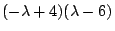 .
Therefore .
Therefore
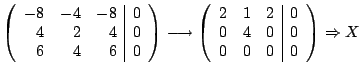
and the eigenvalues are 2, 4, and 6.
To find the eigenvectors, we substitute
 ,
and ,
and
 into
into 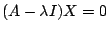 and solve. The resulting equations are
The eigenpairs are
and the eigenspaces are
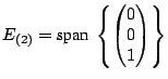
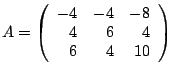
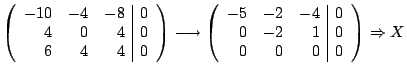
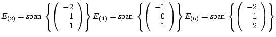
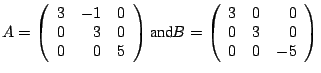
Example The matrices
both have eigenvalues 3 and
 ,
with 3 being an eigenvalue of multiplicity 2. Compare the
eigenspaces for these two matrices.
Solution For
the general eigenpairs are
so the eigenspaces are
For
 the general eigenpairs are
so the eigenspaces for
are
For  (multiplicity of
 ),
while for
, ),
while for
,  (multiplicity
of
). (multiplicity
of
).
a
Remark 32 The eigenvalue of smallest magnitude of a matrix is
the same as the inverse (reciprocal) of the dominant eigenvalue of
the inverse of the matrix. Since most applications of eigenvalues
need the eigenvalue of smallest magnitude, the inverse matrix is
often solved for its dominant eigenvalue. This is why the dominant
eigenvalue is so important.
Also, a bridge in Manchester, England collapsed in 1831 because of
conflicts between frequencies. However, this time, the natural frequency
of the bridge was matched by the frequency caused by soldiers marching
in step. Large oscillations occurred and the bridge collapsed. This is
why soldiers break cadence when crossing a bridge.
Frequencies are also used in electrical systems. When you tune your
radio, you are changing the resonant frequency until it matches the
frequency at which your station is broadcasting. Engineers used
eigenvalues when they designed your radio.
Frequencies are also vital in music performance. When instruments are
tuned, their frequencies are matched. It is the frequency that
determines what we hear as music. Although musicians do not study
eigenvalues in order to play their instruments better, the study of
eigenvalues can explain why certain sounds are pleasant to the ear while
others sound "flat" or "sharp." When two people sing in harmony, the
frequency of one voice is a constant multiple of the other. That is what
makes the sounds pleasant. Eigenvalues can be used to explain many
aspects of music from the initial design of the instrument to tuning and
harmony during a performance. Even the concert halls are analyzed so
that every seat in the theater receives a high quality sound.
Car designers analyze eigenvalues in order to damp out the noise so
that the occupants have a quiet ride. Eigenvalue analysis is also used
in the design of car stereo systems so that the sounds are directed
correctly for the listening pleasure of the passengers and driver. When
you see a car that vibrates because of the loud booming music, think of
eigenvalues. Eigenvalue analysis can indicate what needs to be changed
to reduce the vibration of the car due to the music.
Eigenvalues are not only used to explain natural occurrences, but
also to discover new and better designs for the future. Some of the
results are quite surprising. If you were asked to build the strongest
column that you could to support the weight of a roof using only a
specified amount of material, what shape would that column take? Most of
us would build a cylinder like most other columns that we have seen.
However, Steve Cox of Rice University and Michael Overton of New York
University proved, based on the work of J. Keller and I. Tadjbakhsh,
that the column would be stronger if it was largest at the top, middle,
and bottom. At the points
 of the way from either end, the column could be smaller because the
column would not naturally buckle there anyway. A cross-section of this
column would look like this:
of the way from either end, the column could be smaller because the
column would not naturally buckle there anyway. A cross-section of this
column would look like this:
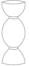
Does that surprise you? This new design was discovered through the
study of the eigenvalues of the system involving the column and the
weight from above. Note that this column would not be the strongest
design if any significant pressure came from the side, but when a column
supports a roof, the vast majority of the pressure comes directly from
above.
Eigenvalues can also be used to test for cracks or deformities in a
solid. Can you imagine if every inch of every beam used in construction
had to be tested? The problem is not as time consuming when eigenvalues
are used. When a beam is struck, its natural frequencies (eigenvalues)
can be heard. If the beam "rings," then it is not flawed. A dull sound
will result from a flawed beam because the flaw causes the eigenvalues
to change. Sensitive machines can be used to "see" and "hear"
eigenvalues more precisely.
Oil companies frequently use eigenvalue analysis to explore land for
oil. Oil, dirt, and other substances all give rise to linear systems
which have different eigenvalues, so eigenvalue analysis can give a good
indication of where oil reserves are located. Oil companies place probes
around a site to pick up the waves that result from a huge truck used to
vibrate the ground. The waves are changed as they pass through the
different substances in the ground. The analysis of these waves directs
the oil companies to possible drilling sites.
There are many more uses for eigenvalues, but we only wanted to give
you a sampling of their uses. When you study science or engineering in
college, you will become quite familiar with eigenvalues and their uses.
There are also numerical difficulties that can arise when data from
real-world problems are used. |

IMPORTANT
RESULTS:
Fact 1
(about homogeneous system of equations):
A system of linear equation is called homogeneous if the right
sides are equal to 0.
Example:
2x + 3y - 4z = 0
x - y + z = 0
x - y = 0
A homogeneous system of equations always has a solution (0,0,...,0). Every
homogeneous system has either exactly one solution or infinitely many solutions.
If a homogeneous system has more unknowns than equations, then it has infinitely
many solutions.
Fact 2(
about nonsingular (invertible) matrices):
If A is an n by n square matrix, then the following
statements are equivalent.
- A invertible (nonsingular)
- The system Av=b has at least one solution for
every column-vector b.
- The system Av=b has exactly one solution for
every column-vector b (here v is the column-vector of
unknowns).
- The system Av=0 has only the trivial solution
(0,0,0,...0)
- The Reduced-echelon-form of A is the identity
matrix n by n.
- A is a product of elementary matrices.
Fact 3 ( about
elementary matrices):
If the elementary matrix E is obtained by performing a row operation
on the identity matrix Im and if A is an m by
n matrix, then the product EA is the matrix obtained from A
by applying the same row operation.
Every elementary matrix is invertible and the inverse is again an elementary
matrix. If an elementary matrix E is obtained from I by using a
certain row-operation q then E-1 is obtained from I
by the "inverse" operation q-1 defined as follows:
· If q is
the adding operation (add x times row j to row i) then q-1
is also an adding operation (add -x times row j to row i).
· If q is
the multiplication of a row by x then q-1 is the
multiplication of the same row by x-1.
· If q is a swapping
operation then q-1=q.
Fact 4( about symmetric
matrices):
- The sum of two symmetric matrices is a symmetric
matrix.
- If we multiply a symmetric matrix by a scalar, the
result will be a symmetric matrix.
- If A and B are symmetric matrices then
AB+BA is a symmetric matrix
- Any power An of a symmetric matrix
A (n is any positive integer) is a symmetric matrix.
- If A is an invertible symmetric matrix then
A-1 is also symmetric.
- If the product of two symmetric matrices A and
B of the same size is symmetric then AB=BA.
- Conversely, if A and B are symmetric
matrices of the same size and AB=BA then AB is
symmetric
Fact 5(about triangular
matrices):
- Every square matrix is a sum of an upper triangular
matrix and a lower triangular matrix.
- The product of two upper (lower) triangular matrices
is an upper (lower) triangular matrix.
- The transpose of an upper triangular matrix is a low
triangular matrix.
Fact 6(about
skew-symmetric matrices):
- If A is invertible and skew-symmetric matrices
then the inverse of A is skew-symmetric.
- If A and B are skew-symmetric matrices
then AT, A+B, AB-BA, and kA are skew-symmetric for
every scalar k.
- Every square matrix is the sum of a symmetric and a
skew-symmetric matrices.
Fact 7(about
Determinant of a matrix):
Let A be an n by n matrix. Then the following conditions
hold.
- If we multiply a row (column) of A by a number,
the determinant of A will be multiplied by the same number.
- If two rows (columns) in A are equal then det(A)=0.
- If we add a row (column) of A multiplied by a
scalar k to another row (column) of A, then the determinant
will not change.
- If we swap two rows (columns) in A, the
determinant will change its sign.
- det(A)=det(AT).
- If A has a zero row (column) then det(A)=0.
- det(AB)=det(A)det(B) for any B, n
by n matrices
- Aadj(A) = det(A)I =adj(A)A.
- If A is invertible (nonsingular) then
A-1 = (1/det(A)) adj(A)
Fact 8(about basis,
dependent, independent)
Let V be a vector space. The following properties of bases of V
hold:
- If S is a basis of a vector space V then every
vector in V has exactly one representation as a linear combination of
elements of S.
- If V has a basis with n elements then
- Every set of vectors in V which has more
than n elements is linearly dependent.
- Every set of vectors with fewer than n
elements does not span V.
- Every set of n independent
vectors in V form a basis for V
- All bases of V have the same number of
elements.
- If V is an n-dimension
space and S is a set of n elements from V. Then S
is a basis of V in each of the following cases:
- S spans V.
- S is linearly
independent.
- If S is a linearly dependent set in an n-dimensional
space V and V=span(S) then by removing some elements of
S we can get a basis of V.
- If S is a linearly independent subset of V
which is not a basis of V then we can get a basis of V by
adding some elements to
- a subset S of a vector space V is
linearly independent if and only if there exists exactly one linear
combination of elements of S which is equal to 0, the one with all
zero coefficients.
- If a subset S of a vector space V
contains 0 then S is linearly dependent.
- A set S with exactly two vectors is linearly
dependent if and only if one of these vectors is a scalar multiple of the
other.
- Let f1, f2,...,fn
be functions in C[0,1] each of which has first n-1 derivatives. The
determinant of the following matrix
|
[ f1(x) |
f2(x) |
.... |
fn(x)
] |
|
[ f'2(x) |
f'1(x) |
.... |
f'n(x)
] |
|
[ f''2(x) |
f''1(x) |
.... |
f''n(x)
] |
|
..................................... |
|
[ f2n-1(x) |
f1n-1(x) |
.... |
fnn-1(x)
] |
is called the Wronskian of this set of functions.
If the Wronskian of this set of functions is not identically zero then the
set of functions is linearly independent (The CONVERSE is not TRUE!!!).
Fact 9(about Linear
Transformations):
1. If T is a linear transformation from V to W then T(0)=0.
2. If T is a linear transformation from V to W and S
is a linear transformation from W to Y (V, W, Y are vector
spaces) then the product (composition) ST is a linear transformation from
V to Y.
3. If T and S are linear transformations from V to W
(V and W are vector spaces) then the sum T+S which takes
every vector A in V to the sum T(A)+S(A) in W is
again a linear transformation from V to W.
4. If T is a linear transformation from V to W and k
is a scalar then the map kT which takes every vector A in V
to k times T(A) is again a linear transformation from V to
W.
5. If T is a linear transformation from Rm
to Rn then dim(range(T))+dim(kernel(T))=m.
6. If [T]B,K is the matrix of a linear Transformation
T from a vector space V into W, then for every vector v in
V we have:
[T(v)]K = [T]B,K[v]B.
Fact 10 (dim(column space of A ) + dim(Nul(A) = number of columns of A):
- For every matrix A the dimension of the column
space plus the dimension of the null space is equal to the number of columns
of A.
2. The column rank and the row rank of every matrix
coincide and they are equal to the (row) rank of the reduced row echelon form
of this matrix, and are equal to the number of leading 1's in this reduced row
echelon form.
Fact 11(about orthogonal vectors):
1. Every set of pairwise orthogonal non-zero vectors is
linearly independent.
Fact 12 (about Eigenvalues, Eigenspaces,
and Diagolization )
Algorithm:
|
To diagonalize an n by n matrix A:
- First solve the eigenvalue problem for
A..
- If there are fewer than n
linearly independent eigenvectors, then A is
not diagonable. Stop.
- Write down the matrices U,
whose columns are the eigenvectors, and D,
which has the eigenvalues on the main diagonal and zeroes
everywhere else. (The order of the eigenvalues in D
must be the same as the order of the eigenvectors in U.)
- Write
A = U D U-1. |
If a square matrix is not diagonable, it is still possible, and useful, to
convert it with a similarity transformation into upper triangular echelon form.
In a course on linear algebra you will study this in more depth. Here we will
just give an example showing what can happen:
Example 5. Let
[ 0 1 1 ]
A := [12 -2 -8 ]
[0 2 2 ]
This matrix has a hidden special property. If you calculate
its cube, you find, somewhat surprisingly, that
3 [ 0 0 0 ]
A = [ 0 0 0 ]
[ 0 0 0 ]
Now, what could the eigenvalues of such a nilpotent
matrix be? If Av = v,
then
A3 v = 3v
and we conclude that the only possible eigenvalue is 0. But
if a basis of three eigenvectors all have eigenvalue zero, then the whole matrix
A must be the zero matrix. It isn't.
Let's illustrate why diagonalizing is useful with another
Model problem. Let
[ 3 -5]
A = [-5 3].
Find A10.
Solution. Don't just multiply! Instead, first
diagonalize:
A = U-1D U,
where by following the algorithm we find:
1
= -2, with eigenvector
[ 1]
v = [ 1].
1
and
1
= 8, with eigenvector
[ 1]
v = [-1].
2
Therefore,
[1/2 1/2] [2 0] [ 1 1] -1
A = [1/2 -1/2] [0 8] [ 1 -1] =: U D U .
Now, we notice that the product of A with itself p
times collapses:
Ap = U D U-1
U D U-1 ... U D U-1
= U D D ...D U-1,
because U-1 U = I_n. Therefore the
answer is:
6 [1/2 1/2] [26 0] [ 1 1] [131104 -131040]
A = [1/2 -1/2] [0 86] [ 1 -1] = [-131040 131104].
Now we state and prove the theorem which the last example illustrates.
Tests for diagonalization: :
|
An n by n matrix A can be
diagonalized if any of the following conditions can be verified:
- if all the eigenvalues are different;
or
- if A is "symmetric", that
is, AT = A; or
- if A is "normal", that
is, A AT = AT A.
|
- System of linear equations
- Solution of a system of linear equations
- A
consistent system of equations
- General solution of a system of linear equations
- Augmented matrix of a system of linear equations
- Row operations on matrices
- Equivalent Matrices
- Row-echelon form
- Reduced row-echelon form
- Gauss-Jordan elimination procedure
- Homogeneous system of linear equations
Sum of
matrices
- Multiplying a matrix by a scalar
- Product of matrices
- Identity matrix
- Transpose of a matrix
- Trace
of a matrix
- Invertible matrix
- Inverse of a matrix
- Elementary matrix
- Row-Equivalent
matrices
- Symmetric matrices
- Diagonal matrices
- Upper- and lower-triangular matrices
- Skew-symmetric matrices
- Cofactor of entry aij.
- Determinant of a square matrix
- Cofactor expansion along a row (column)
- The
adjoint of a matrix
- Cramer's rule
- Vector space
- Subspace of a vector space.
- Linear combination of vectors
- Vector space spanned by a set of vectors
- Linearly independent sets of elements in a vector space.
- Linearly dependent sets of elements in a vector space.
- A basis
of a vector space
- The
dimension of a vector space
- The
null space of a matrix
- Nullity of a matrix
- Rank
of a matrix
- Row Space of a Matrix
- Column space of a matrix
- The
Wronskian of a set of functions
- Linear transformations
- Kernel
and Range of a linear transformation
- Coordinates of a vector in a given basis
-
Standard matrix
representation of a linear transformation
-
Eigenvector, eigenvalue,
eigenspace, and
the characteristic polynomial of a matrix
-
Similar matrices
-
Diagonalizable
Matrix
-
Orthogonal vectors
-
Orthogonal basis
-
Gram-Schmidt procedure
Definitions in Linear Algebra:
(for examples click here)
A system of linear equations
is any sequence of linear equations. A
solution of a system
of linear equations is any common solution of these equations. A
system is called consistent if it has a solution.
A
general solution of a system of linear
equations is a formula which gives all solutions for different values of
parameters.
Examples. 1. Consider the system:
                                          x +  y =  7
                                         2x + 4y = 18
This system has just one solution: x=5, y=2.
This is a general solution of the system.
2. Consider the system:
                                       x +  y + z =  7
                                      2x + 4y + z = 18.
This system has infinitely many solutions given by this formula:
                                        x = 5 - 3s/2
                                        y = 2 + s/2
                                        z = s
This is a general solution of our system.
Two matrices are said to be
row-equivalent if one can be obtained from
the other by a sequence (order may vary) of
elementary row operations
given below.
(Also see
row-equivalent (2))
* Interchanging two rows
* Multiplying a row by a non zero constant
* Adding a multiple of a row to another row
Row-Echelon Form and Reduced Row-Echelon Form
A matrix in row-echelon form
has the following
properties.
1. All rows consisting entirely of zeros occur at the
bottom of the matrix
2. For each row that does not entirely consist of zeroes, the first non zero
entry is 1 – called a leading 1.
3. For two successive non zero rows, the leading 1 in the higher row is
farther to the left that the leading 1 in the lower row.
A matrix in row-echelon form is in
reduced
row-echelon form if every column that has a leading 1 has zeros in every
position above and below its leading 1.
Augmented Matrix
A matrix derived from a system of linear equations is
called the augmented matrix of the system.
Example Consider the system of equations:
                       x1 + 2x2 +         x4   =  6
                                     x3 +  6x4  =  7
                                                 x5=1
Its augmented matrix is
| [ 1 |
2 |
0 |
1 |
0 |
6 ] |
| [ 0 |
0 |
1 |
6 |
0 |
7 ] |
| [ 0 |
0 |
0 |
0 |
1 |
1 ] |
The matrix has the reduced row echelon form. The leading unknowns are x1,
x3 and x5; the free unknowns are x2 and
x4. So the general solution is:
                              x1= 6-2t-s
                              x2= s
                              x3= 7-6t
                              x4= t
                              x5= 1
If the augmented matrix does not have the reduced row echelon form but has
the (ordinary) row echelon form then the general solution also can be easily
found.
The method of finding the solution is called the back-substitution.
First we solve each of the equations for the leading unknowns The last
non-zero equation gives us the expression for the last leading unknown in terms
of the free unknowns. Then we substitute this leading unknown in all other
equations by this expression. After that we are able to find an expression for
the next to the last leading unknown, replace this unknown everywhere by this
expression, etc. until we get expressions for all leading unknowns. The
expressions for leading unknowns that we find in this process form the general
solution of our system of equations.
Example. Consider the following system of equations.
                    x1-3x2+ x3-x4 = 2
                         x2+2x3-x4 = 3
                              x3+x4 = 1
Its augmented matrix
| [ 1 |
-3 |
1 |
-1 |
2 ] |
| [ 0 |
1 |
2 |
-1 |
3 ] |
| [ 0 |
0 |
1 |
1 |
1 ] |
is in the row echelon form.
The leading unknowns are x1, x2, x3;
the free unknown is x4.
Solving each equation for the leading unknown we get:
                            x1=2+3x2-x3+x4
                            x2=3-2x3+x4
                            x3=1-x4
The last equation gives us an expression for x3: x3=1-x4.
Substituting this into the first and the second equations gives:
                    x1=2+3x2-1+x4+x4=1+3x2+2x4
                    x2=3-2(1-x4)+x4=1+3x4
                    x3=1-x4
Now substituting x2=1+3x4 into the first equation,
we get
                    x1=1+3(1+3x4)+2x4=4+11 x4
                    x2=1+3x4
                    x3=1-x4
Now we can write the general solution:
                                    x1=4+11 s
                                    x2=1+ 3 s
                                    x3=1-   s
                                    x4=     s
Let us check if we made any arithmetic mistakes. Take x4=1 and
compute x1=15, x2=4, x3=0, x4=1.
Substitute it into the original system of equations:
                            15 - 3 * 4 + 0 - 1 = 2
                                 4 + 2 * 0 - 1 = 3
                                         0 + 1 = 1
OK, it seems that our solution is correct.
Consistent System
A system of linear equations which has a solution.
Homogeneous System
A homogeneous system of linear equations is of the form:
a11x1
+ a12x2
+ . . . + a1nxn=0
a21x1
+ a22x2
+ . . . + a2nxn=0
am1x1
+ am2x2
+ . . . + amnxn=0
That is, a homogeneous system of linear equations has all constant terms
equal to zero.
The Gauss-Jordan
elimination procedure
There exists a standard procedure to obtain a reduced row echelon matrix from
a given matrix by using the row operations.
This procedure consists of the following steps.
- Locate the leftmost column which does not consist of zeroes.
- If necessary swap the first row with the row which contains a non-zero
number a in the column found on step 1.
- If this number a is not 0, multiply the first row by 1/a, to get a
leading 1 in the first row.
- Use the first row to make zeroes below the leading 1 in the first row
(by using the adding operation).
- Cover the first row and apply the first 4 steps to the remaining
sub-matrix. Continue until the whole matrix is in the row echelon form.
- Use the last non-zero row to make zeroes above the leading 1 in this
row. Use the second to last non-zero row to make zeroes above the leading 1
in this row. Continue until the matrix is in the reduced row echelon form.
Row Equivalent Matrices
Two matrices A and B are row equivalent if A is a product of elementary
matrices times B, or equivalently if A can be obtained from B by a finite
sequence of elementary row operations.
In order to multiply a matrix
by a scalar, one has to multiply all entries of the matrix by this
scalar.
Example:
| 3 * |
| [ 2 |
3 |
1 |
2 ] |
| [ 3 |
1 |
0 |
1 ] |
| [ 1 |
2 |
2 |
3 ] |
|
= |
| [ 6 |
9 |
3 |
6 ] |
| [ 9 |
3 |
0 |
3 ] |
| [ 3 |
6 |
6 |
9 ] |
|
Pruduct
of two matrices:
The product of a row-vector v of size (1, n) and a column
vector u of size (n,1) is the sum of products of corresponding
entries:
uv=u(1)v(1)+u(2)v(2)+...+u(n)v(n)
Example:
                        3
            (1, 2, 3) * 4 =1*3 + 2*4 + 3*1 = 3+8+3=14
                        1
Example:
                        x
            (2, 4, 3) * y = 2x + 4y + 3z
                        z
As you see, we can represent the left side of a linear equation as a product
of two matrices. The product of arbitrary two matrices which we shall define
next will allow us to represent the left side of any system of equations as a
product of two matrices.
Let A be a matrix of size (m,n), let B be a matrix of
size (n,k) (that is the number of columns in A is equal to
the number of rows in B. We can subdivide A into a column of m
row-vectors of size (1,n). We can also subdivide B into a row of
k column-vectors of size (n,1):
          r1
          r2
       A =...      B=[c1 c2 ... ck]
          rm
Then the product of A and B is the matrix C
of size (m,k) such that
C(i,j)=ricj
(C(i,j) is the product of the row-vector ri and the
column-vector cj).
Matrices A and B such that the number of columns of A
is not equal to the number of rows of B cannot be multiplied.
Example:
Example:
|
|
* |
|
= |
| [ 2x + 3y + 4z ] |
| [ x + 2y + 3z ] |
|
You see: we can represent the left part of a system of linear equations as a
product of a matrix and a column-vector. The whole system of linear equations
can thus be written in the following form:
AX = b
Identity Matrix I_n:
Let In denote the identity matrix of order n
that is a square matrix of order n with 1s on the main diagonal and
zeroes everywhere else. Then for every m by n matrix A the
product of A and In is A and the product of Im
and A is A.
Nonsingular (invertible) matrices:
A
square matrix of size n A is called invertible
(nonsingular) if there exists a square matrix B of the same size
such that AB = BA = In, the
identity matrix of size n. In this case B is called the
inverse of A and B is denoted by A-1.
FINDING THE INVERSE OF A MATRIX
Let A be square matrix order n.
1. Write a matrix that consists of the given matrix A
on the left and the identity matrix n x n next to A on the
right, separating the matrices A and I by a (vertical) dotted line
to obtain [A:I].
2. If possible, row reduce A to I using elementary row
operations on the matrix [A:I]. The result will be the matrix [I:A-1].
Note that for some matrices an inverse does not exist. If it is not possible to
obtain [I:A-1], then the matrix A is not invertible.
3. Check your work by multiplying to see that AA-1 = I
= A-1 A.
An elementary matrix is a matrix obtained from an identity
matrix by one of the row-operations.
Example.
|
|
, |
|
[ 1 |
0 |
0 ] |
|
[ 1 |
1 |
0 ] |
|
[ 0 |
0 |
1 ] |
|
, |
|
[ 1 |
0 |
0 ] |
|
[ 0 |
0 |
1 ] |
|
[ 0 |
1 |
0 ] |
|
, |
|
[ 1 |
0 |
0 ] |
|
[ 0 |
2 |
0 ] |
|
[ 0 |
0 |
1 ] |
|
The first two matrices are obtained by adding a multiple of one row to
another row. The third matrix is obtained by swapping two rows. The last matrix
is obtained by multiplying row by a number.
As we see, elementary matrices usually have lots of zeroes.
Elementary matrices which are obtained by adding rows contain only one
non-diagonal non-zero entry.
Elementary matrices which are obtained by multiplying a row by a number
contain exactly 1 non-unit entry on the diagonal and no non-zero entries outside
the diagonal.
Elementary matrices which are obtained by swapping consist of 0s and 1s and
contain exactly 2 non-diagonal entries.
The converse statements are true also (for example every matrix with 1s on
the diagonal and exactly one non-zero entry outside the diagonal) is an
elementary matrix.
The main result about elementary matrices
is that every invertible matrix is a product of elementary matrices. These are
in some sense the smallest particles in the world of invertible matrices.
Transpose of a matrix:
If A is any m by n matrix then the transpose
of A, denoted by AT, is defined to be the n by
m matrix obtained by interchanging the rows and columns of A, that
is the first column of AT is the first row of A, the
second column of AT is the second row of A, etc.
Example.
The transpose of
Trace of a
Matrix:
If A is a square matrix of size n
then the sum of the entries on the main diagonal of A is called the
trace of A and is denoted by tr(A).
Example.
The trace of the matrix
| [ 1 |
2 |
3 ] |
| [ 4 |
5 |
6 ] |
| [ 7 |
8 |
9 ] |
is equal to 1+5+9=15
A square matrix A is called symmetric if AT=A,
that is if A(i,j)=A(j,i) for every i and j. Thus A
is symmetric if and only if it is symmetric with respect to the main diagonal.
Here is an example of a symmetric matrix:
|
[ 1 |
2 |
3 ] |
|
[ 2 |
4 |
5 ] |
|
[ 3 |
5 |
6 ] |
An important subclass of symmetric matrices is formed by diagonal
matrices, i.e. matrices which have zeroes everywhere outside the main diagonal.
For example, the identity matrix is a diagonal matrix.
A square matrix A is called upper triangular (resp.
lower triangular) if all its entries below (resp. above) the main
diagonal are zeroes, that is A(i,j)=0 whenever i is greater than
j (resp. A(i,j)=0 whenever i is less than j).
Example.
|
[ 1 |
2 |
3 ] |
|
[ 0 |
0 |
1 ] |
|
[ 0 |
0 |
1 ] |
|
, |
|
[ 1 |
0 |
0 ] |
|
[ 0 |
1 |
0 ] |
|
[ 2 |
3 |
4 ] |
|
The first of these matrices is upper triangular, the second is lower
triangular.
A square matrix A is called skew-symmetric
if A^T = -A, that is A(i,j)=-A(j,i) for every i and j.
In particular, if i=j then A(i,i)=0, that is the diagonal entries
of a skew-symmetric matrix are equal to 0.
Example:
|
[ 0 |
2 |
3 ] |
|
[ -2 |
0 |
4 ] |
|
[ -3 |
-4 |
0 ] |
Determinant:
Let Aij is the cofactor of entry a_ij
that is equal to (-1)i+j multiplied by
the determinant of the matrix obtained from A by deleting the i-th
row and the j-th column (the determinant of this smaller matrix has a
special name also; it is called the minor of entry A(i,j)).
-
For every i=1,...,n we have det(A)=a_i1
Ai1 + a_i2 Ai2 +...+ a_in Ain This
is called the cofactor expansion of det(A) along the i-th row
(a similar statement holds for columns).
-
The determinant of a triangular matrix is the product of
the diagonal entries.
Adjoint Matrix:
Definition. If A is any n by n matrix and Aij
is the cofactor of a_ij then the matrix
|
[ A11 |
A21 |
... |
An1 ] |
|
[ A12 |
A22 |
... |
An2 ] |
|
............................ |
|
[ A1n |
A2n |
... |
Ann ] |
is called the adjoint of A, denoted adj(A).
(Notice that this matrix is obtained by replacing each entry of A by
its cofactor and then taking the transpose.)
(Cramer's rule) If A is an invertible matrix then the
solution of the system of linear equalitions
AX=b
can be written as
x1=det(A1)/det(A), x_2 = det(A_2)/Det(A)...
...,
xn= det(An)/det(A)
where Ai is the matrix obtained from A
by replacing the i-th column by the column vector b.
VECTOR SPACE :
Any set of objects V where addition
and scalar multiplication are defined and satisfy properties 1--7 is called
a vector space. Let A, B, C be elements
in V, and a, b be real numbers:
-
The addition is commutative and associative: A+B=B+A,
A+(B+C)=(A+B)+C
-
The multiplication by scalar is distributive with respect to
the addition: a(B+C)=aB+aC
-
The product by a scalar is distributive with respect to the
addition of scalars: (a+b)C=aC+bC
-
a(bC)=(ab)C
-
1*A=A (here 1 is the scalar 1)
-
There exists a zero n-vector 0 such that
0+A=A+0=A for every A
-
0*A=0 (here the first 0 is the scalar 0, the second 0
is the zero-vector)
Continuous functions, matrices, R^n, P_n, and (complex
numbers )satisfy the abave properties.
Of course, we denote B+(-A) as B-A, so the
subtraction is a derived operation, we derive it from the addition
and the multiplication by scalar. Notice that in the solution of the equation
X+A=B we did not use the fact that A,B,X are functions or vectors (or
matrices or numbers for that matter), we used only the properties of our basic
operations.
Here by addition we mean any operation which
associates with each pair of objects A and B from V another
object (the sum) C also from V; by a scalar multiplication
we mean any operation which associates with every scalar k and every
object A from V another object from V called the
scalar multiple of A and denoted by kA.
Elements of general vector spaces are usually called
vectors. For any system of vectors A1,...,An
and for any system of numbers a1,...,an one can
define a linear combination of A1,...,An
with coefficients a1,...,an as
a1A1+...+anAn.
Notice that a vector space does not necessarily consist of
n-vectors or vectors on the plane. The set of continuous functions, the set of
k by n matrices, the set of complex numbers are examples of vector
spaces.
Not every set of objects with addition and scalar multiplication
is a vector space. For example, we can define the following operations on the
set of 2-vectors:
Addition: (a,b)+(c,d)=(a+c,d).
Scalar multiplication: k(a,b)=(k2a,b).
Then the resulting algebraic system will not be a vector space
because if we take k=3, m=2, a=1, b=1 we have:
(k+m)(a,b)=(3+2)(1,1)=5(1,1)=(25,1); k(a,b)+m(c,d)=3(1,1)+2(1,1)=(9,1)+(4,1)=(13,1),
Thus the third property of vector spaces does not hold.
Let V be a vector space . A subset W of V is called a
subspace of V if W is closed under
addition and scalar multiplication, that is if for every vectors A and
B in W the sum A+B belongs to W and for every vector
A in W and every scalar k, the product kA belongs to
W.
Positive Examples.
1. The whole space Rn is a subspace of itself. And the set
consisting of one vector, 0, is a subspace of any space.
2. In R2, consider the set W of all vectors which
are parallel to a given line L. It is clear that the sum of two vectors
which are parallel to L is itself parallel to L, and a scalar
multiple of a vector which is parallel to L is itself parallel to L.
Thus W is a subspace.
3. A similar argument shows that in R3, the set W of
all vectors which are parallel to a given plane (line) is a subspace.
4. The set of all polynomials is a subspace of the space of continuous
functions on [0,1], C[0,1]. The set of all polynomials whose degrees do
not exceed a given number, is a subspace of the vector space of polynomials, and
a subspace of C[0,1].
5. The set of differentiable functions is also a
subspace of C[0,1].
Negative Examples.
1. In R2, the set of all vectors which are parallel to one
of two fixed non-parallel lines, is not a subspace. Indeed, if we take a
non-zero vector parallel to one of the lines and add a non-zero vector parallel
to another line, we get a vector which is parallel to neither of these lines.
2. The set of polynomials of degree 2 is not a subspace of C[0,1].
Indeed, the sum of x2+x and -x2 is a
polynomial of degree 1.
Linear Combination
A linear combination of the vectors v1, v2,
. . . ,vn is a vector w of the
form
w = α1v1 + α2v2
+ . . . + αnvn .
Spanning set:
Let
v1,
v2,
. . . ,vn
be elements of a vector space V. Then Span{ v1,
v2,
. . . ,vn }
is the set ofall possible linear combination of the elements
v1,
v2,
. . . ,vn .
It is easily verified that
Span{ v1,
v2,
. . . ,vn }
is a subspace of V (i.e.
Span{ v1,
v2,
. . . ,vn }
is a vector space).
Linearly Independent
, Linearly Dependent:
A subset S of a vector space V is called linearly
independent if no element of S is a linear combination of other
elements of S.
A subset S of a vector space is called linearly dependent
if it is not linearly independent.
Notice that if a subset of a set S is linearly dependent then the
whole set is linearly dependent (the proof is an exercise).
Examples.
1. Every two vectors in the line R are linearly dependent (one vector is
proportional to the other one).
2. Every three vectors on a plane R2 are linearly
dependent. Indeed, if two of these vectors are parallel then
3. If a subset S of Rn consists of more than n
vectors then S is linearly dependent. ( )
4. The set of polynomials x+1, x2+x+1, x2-2x-2, x2-3x+1
is linearly dependent. To prove that we need to find numbers a, b, c, d
not all equal to 0 such that
a(x+1)+b(x2+x+1)+c(x2-2x-2)+d(x2-3x+1)=0
This leads to a homogeneous system of linear equations with 4 unknowns and 3
equations. Such a system must have a non-trivial solution by a result
about homogeneous systems of linear equations.
Wronskian
Let f1, f2,...,fn be functions in
C[0,1] each of which has first n-1 derivatives. The determinant of the following
matrix
| [ f1(x) |
f2(x) |
.... |
fn(x) ] |
| [ f'2(x) |
f'1(x) |
.... |
f'n(x) ] |
| [ f''2(x) |
f''1(x) |
.... |
f''n(x) ] |
| ..................................... |
| [ f2n-1(x) |
f1n-1(x) |
.... |
fnn-1(x) ] |
is called the Wronskian of this set of functions.
Theorem. Let f1, f2,...,fn be
functions in C[0,1] each of which has first n-1 derivatives. If
the Wronskian of this set of functions is not identically zero then the set of
functions is linearly independent.
Basis, Rank,
and dimension:
A set S of vectors in a vector space V is called a basis
if
- S is linearly independent and
- V=span(S), that is every vector in V is
a linear combination of vectors in S.
A dimension of a vector space V (denoted by dim(V)
), is the number of elements in a basis for V. There is one exception of
this definition: the dimension of the zero space (the vector space consisting of
one vector, zero) is defined to be 0 and not 1.
Let S be a set of vectors in a vector space. Then the dimension of the
vector space spanned by S is called the rank of S.
If A is a matrix then the rank of the set of its columns is called the
column rank of A and the rank of the set of its rows is called the
row rank of A.
It is known that the column rank of A is equal to the row rank of
A for every matrix a.
Column Space
The column space of an mxn matrix A is the span of the columns of A and is
denoted by col(A).
Row Space
The row space of a matrix A is the span of the rows of A and is denoted by
row(A).
Nullspace (or Kernel)
The nullspace of an mxn matrix A is null(A) = {x
∈ Rn such that Ax
= 0}.
Nullity
The nullity of a matrix A is the dimension of the nullspace of A.
nullity(A) = dim(null(A))
Let V and W be arbitrary vector spaces. A
map T from V to W is called a linear transformation
if
- For every two vectors A and B in V
T(A+B)=T(A)+T(B);
- For every vector A in V and every number
k
T(kA)=kT(A).
In the particular case when V=W, T
is called a linear operator in V.
Positive examples.1. Let V be the set of all polynomials in one
variable. We shall see later that V is a vector space with the natural
addition and scalar multiplication (it is not difficult to show it directly).
The map which takes each polynomial to its derivative is a linear operator in
V as easily follows from the properties of derivative:
(p(x)+q(x))' =
p'(x) +q'(x),
(kp(x))'=kp'(x).
2. Let C[0,1] be the vector space of all continuous functions on the
interval [0,1]. Then the map which takes every function S(x) from C[0,1]
to the function h(x) which is equal to the integral from 0 to x of
S(t) is a linear operator in C[0,1] as follows from the properties
of integrals.
int(T(t)+S(t))
dt = int T(t)dt + int S(t)dt
int kS(t) dt = k int S(t) dt.
3. The map from C[0,1] to R which takes every function S(x)
to the number S(1/3) is a linear transformation (1/3 can be replaced by
any number between 0 and 1):
(T+S)(1/3)=T(1/3)+S(1/3),
(kg)(1/3)=k(S(1/3)).
4. The map from the vector space of all complex numbers C to
itself which takes every complex number a+bi to its imaginary part
bi is a linear operator (check!).
5. The map from the vector space of all n by n matrices (n
is fixed) to R which takes every matrix A to its (1,1)-entry A(1,1)
is a linear transformation (check!).
6. The map from the vector space of all n by n matrices to R
which takes every matrix A to its trace trace(A) is a linear
transformation .
7. The map from an arbitrary vector space V to an arbitrary vector
space W which takes every vector v from V to 0 is a linear
transformation . This transformation is called the
null transformation
8. The map from an arbitrary vector space V to V which takes
every vector to itself (the identity map) is a linear operator (check!). It is
called the identity operator,
denoted I.
Negative examples. 1. The map T from which takes every function
S(x) from C[0,1] to the function S(x)+1 is not a
linear transformation because if we take k=0, S(x)=x then the
image of kT(x) (=0) is the constant function 1 and k times the
image of T(x) is the constant function 0. So the second property of
linear transformations does not hold.
kernels and ranges
of linear transformations
Sources of subspaces: kernels and ranges
of linear transformations
Let T be a linear transformation from a vector space V to a
vector space W. Then the kernel of T is the set of
all vectors A in V such that T(A)=0, that is
ker(T)={A in V
| T(A)=0}
The range of T is the set of all vectors in W
which are images of some vectors in V, that is
range(T)={A in W |
there exists B in V such that T(B)=A}.
Notice that the kernel of a transformation from V to W
is a subspace of V and the range is a subspace of W. For example
if T is a transformation from the space of functions to the space of real
numbers then the kernel must consist of functions and the range must consist of
numbers.
Coordinate of a vector in a given basis:
Let S be a basis of a vector space V and let a be a
vector from V. Then a can be uniquely represented as a
linear combination of elements from S. The coefficients of
this linear combination are called the coordinates of a in the basis S, we
use the notation
[a]S To denote the coordinates of a in the basis
S
Example.
Vectors (1,2) and (2,3) form a basis of R2 . The vector (4,7)
is equal to the linear combination 2(1,2)+(2,3). Thus the vector (4,7) has
coordinates 2, 1 in the basis of vectors (1,2) and (2,3), we write
[(4, 7)]S =
[2 1]. The same vector has coordinates 4 and 7 in the basis of vectors D =
(1,0) and (0,1). Thus a vector has different coordinates in different bases.
It is sometimes very important to find a basis where the vectors you are dealing
with have the simplest possible coordinates.
Let B={b1,...,bn} be a basis in an
n-dimensional vector space V and K = {d1,...,dm} be a basis in an
m-dimensional vector space W . For every vector v in V
let [v]B denote the column vector of coordinates of v
in the basis B.
Let T be a linear Transformation from V into W. Since T(b1),...,T(bn)
are in W, each of these vectors is a linear combination of vectors from
K. Consider the m by n matrix [T] B,K whose
columns are the column vectors of coordinates [T(b1)]K,...,
[T(bn)]K. This matrix is called the matrix of
the linear operator T in the basis B and K.
Important Result : If [T]B,K is the matrix of a
linear Transformation T from a vector space V
into W, then for every vector v in V
we have:
[T(v)]K = [T]B,K*[v]B.
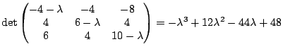
Characteristic Polynomial
The characteristic polynomial of a square matrix A is defined by
p(x) = det(xI - A).
Eigenvalue
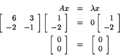
The scalar λ is said to be an eigenvalue of an nxn matrix A if there is a
nonzero vector x with Ax = λx , the eigenvalues of a
matrix A, n by n, are found by setting the characteristic polynomial of
A equals to zero.
A non-zero vector w is called an
eigenvector of a matrix A with the eigenvalue a
if Aw=aw (and hence a is an eigenvalue of A that
corresponds to the eigenvector w.)
We can rewrite the equality Aw=aw in the following form:
Aw=aIw
where I is the identity matrix. Moving the right hand side to the
left, we get:
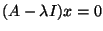
(A-aI)w=0
This is a homogeneous system of linear equations. If the matrix A has
an eigenvector W then this system must have a non-trivial solution (w
is not 0 !). this is equivalent to the condition that the matrix A-aI
is not invertible, and this is equivalent to the condition that det(A-aI)
is equal to zero. Thus a matrix A has an eigenvector with an
eigenvalue a if and only if det(A-aI)=0.
Notice that det(A-xI) is a polynomial with the unknown x.
This polynomial is called the characteristic polynomial of the
matrix A.
Thus in order to find all eigenvectors of a matrix A, one needs to
find the characteristic polynomial of A, find all its roots (=eigenvalues)
and for each of these roots a, find the solutions of the homogeneous
system (A-aI)w=0.
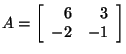
Example.
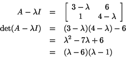
Let A be the matrix
The characteristic polynomial det(A-xI) is (1-x)2-4.
The roots are x=-1 and x=3. These are the eigenvalues A.
Let a=-1. Then the system of equations (A-aI)w=0 has the form
2x+2y=0
2x+2y=0
where w=(x,y). The general solution is:
x=-t
y=t
This solution gives the set of all eigenvalues with the eigenvalue -1. It is
a subspace spanned by the vector b1=(-1,1).
Now let a=3. Then the system (A-aI)w=0 has the form
-2x+2y=0
2x-2y=0
The general solution is:
                                                x = t

                                                y = t
Thus the set of eigenvectors with eigenvalue 3 forms a subspace spanned by
the vector (1,1).
Eigenvector : The nonzero vector x is said to be an eigenvector of the matrix A,
associated with the eigenvalue λ if Ax = λx. Thus in order
to find all eigenvectors of a matrix A, one needs to find the
characteristic polynomial of A, find all its roots (=eigenvalues) and for
each of these roots a, find the solutions of the homogeneous system
(A-aI)v=0.
Eigenspace : The eigenspace associated with the eigenvalue λ of a matrix A is defined by
Eλ = null(λI - A).
Similar Matrices
Matrices A and B are said to be similar if there exists an invertible matrix
S such that
A = S-1BS.
Diagonalizable Matrix
A square matrix A is said to be diagonalizable if there is an invertible
matrix P so that
P-1AP is a diagonal matrix.
Orthogonal Vectors
The vectors u and v in Rn are
said to be orthogonal if u•v (u dot product v)
= 0.
The vectors u and v in an inner product
space are said to be orthogonal if <u,v> = 0.
Notation for both of these is u
⊥ v.
Orthonormal Vectors
Vectors are said to be orthonormal if they are pairwise orthogonal and are
all unit vectors.
Orthogonal Basis
A set of vectors B is said to be an orthogonal basis for a subspace V if:
1) the vectors in B form a basis for V
2) the vectors in the set are pairwise orthogonal
Gram-Schmidt procedure:
(Orthogonal bases. The
Gram-Schmidt algorithm)
A basis of a vector space is called orthogonal if the
vectors in this basis are pairwise orthogonal.
A basis of a Euclidean vector space ( think of
R^n, and if x, y in R^n, then <x, y>
means the dot product of x with y, i.e <x, y> = x..y
) is called orthonormal if it is orthogonal and each vector
has norm 1.
Given an orthogonal basis {v1,...,vn}, one can
get an orthonormal basis by dividing each vi by its length: {v1/||v1||,...,vn/||vn||}.
Suppose that we have a (not necessarily orthogonal) basis {s1,...,sn}
of a Euclidean vector space V. The next procedure, called the
Gram-Schmidt algorithm, produces an orthogonal basis {v1,...,vn}
of V. Let
v1=s1
We shall find v2 as a linear combination of v1
and s2: v2=s2+xv1.
Since v2 must be orthogonal to v1, we have:
0=v2v1=(s2+xv1)v1=s2v1
+ x<v1,v1>.
Hence
x=-<s2,v1>/<v1,v1>,
so
v2=s2-(<s2,v1>/<v1,v1>)
v1
Next we can find v3 as a linear combination of s3,
v1 and v2. A similar calculation gives that
v3=s3 - (<s3,v1>/<v1,v1>)
v1 - (<s3,v2>/<v2,v2>) v2.
Continuing in this manner, we can get the formula for vi+1:
vi=si - (<si,v1>/<v1,v1>)
v1 - (<si,v2>/<v2,v2>) v2-...-(<si,vi-1>)/<vi-1,vi-1>)
vi-1
By construction, the set of vectors {v1,...,vn}
is orthogonal. None of these vectors is 0. Indeed, if vi were
equal to 0 then si, v1,...,vi-1 would be
linearly dependent, which would imply that s1,...,si
are linearly dependent (replace each vj as a linear
combination of s1,...,sj), which is impossible
since {s1,...,sn} is a basis. This implies that {v1,...,vn}
are linearly independent. Since {v1,...,vn} is an
orthogonal basis , one can get an orthonormal basis by dividing each vi
by its length: {v1/||v1||,...,vn/||vn||}
is an orthonormal basis.
 is a polynomial
  .
.
 is an eigenvalue, any nontrivial solution of
 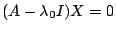 is an eigenvector of
 (that is, if
  ) and
) and  is an eigenpair of
 is an eigenpair of
 is diagonalizable, then
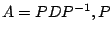 is a matrix whose columns are eigenvectors, and the diagonal entries of
 are the eigenvalues corresponding column by column to their respecctive
eigenvectors.
are the eigenvalues corresponding column by column to their respecctive
eigenvectors.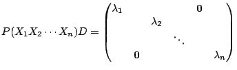


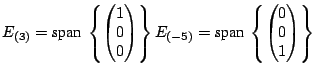
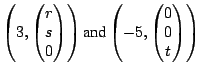
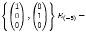 span
span
